DSUS 5 Errata

General

Bayes factors

In print runs up to Feb 2020, I denote Bayes factors as BF₀₁, but the way I describe Bayes factors the correct way to denote the Bayes Factor is BF₁₀ (not the subscript has changed). Page 131 imagine that

You could also report Bayes factors, which are denoted by BF₁₀.

reads as

You could also report Bayes factors, which are denoted by BF₁₀ in the form that I have described them (i.e., when a value greater than 1 is evidence for the alternative hypothesis). Alternatively, the Bayes factor can be expressed as the reciprocal of the value I have described, which reverses the interpretation (i.e., a value greater than 1 is evidence for the null hypothesis) and this form is denoted as BF₀₁ (note the order of the subscripts has changed).

Then on pages 131, 477 & 862 all instances of BF₀₁ should be BF₁₀. This should be corrected in editions printed from Spring 2020 onwards.

Chapter 3

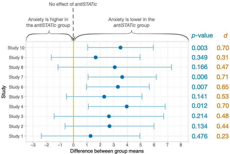
Figure 3.2: In print runs up to Feb 2020, the p-values and values of d are mistakenly listed in reverse order. For example, the values of p = 0.476 and d = 0.23 listed for study 10 are in fact the values for study 1, and the values of p = 0.003 and d = 0.70 listed for study 1 are in fact the values for study 10. You need to mentally reverse the order of those values. That’s quite a challenge (and one I didn’t intend to set you) so here’s the correct figure:

Chapter 5

Query from Floris Hegger

In chapter 4, you discuss several types of graphs. One of them is the grouped scatterplot in which you show how men and women differ in terms of exam performance and exam anxiety. You literally say the following: “These lines (Figure 4.36) tell us that the relationship between exam anxiety and exam performance was slightly stronger in males (the line is steeper) indicating that men’s exam performance was more adversely affected by anxiety than women’s exam anxiety.” I have to (partly) disagree with this. The steepness of the line does not indicate how strong the relationship between the variables is; the strength of a relationship is usually displayed by r, the correlation coefficient. I think it is misleading, since the strength of the relationship is determined by ‘how close the dots are on the line’ and not by ‘the steepness of the line’.

This point is fair, stronger associations do reflect data that cluster more closely around the line, but as Floris also points out the strength of a relationship is usually displayed by r, the correlation coefficient and in the case of two variables, r has a direct relationship to b (the gradient of the line). Therefore, the gradient (slope of the line) provides information about strength but it is ‘contaminated’ by information about the spread of scores. The issue here (and the sense in which the point is a very good one) is that I’ve plotting the raw data not the standardized data. If I’d plotted the standardized data, r would be equal to the gradient. In this situation we could directly compare the male and female lines and use the gradient as information about the relative strength of the relationship in those two groups. However, because I’ve plotted the raw data, the statement in the book only holds if the standard deviations of both variables are the same for males and females, which they might not be.